Code
library(tidymodels)
library(tidyverse)
library(palmerpenguins)
library(tidymodels)
library(tidyverse)
library(palmerpenguins)glimpse(penguins)Rows: 344
Columns: 8
$ species <fct> Adelie, Adelie, Adelie, Adelie, Adelie, Adelie, Adel…
$ island <fct> Torgersen, Torgersen, Torgersen, Torgersen, Torgerse…
$ bill_length_mm <dbl> 39.1, 39.5, 40.3, NA, 36.7, 39.3, 38.9, 39.2, 34.1, …
$ bill_depth_mm <dbl> 18.7, 17.4, 18.0, NA, 19.3, 20.6, 17.8, 19.6, 18.1, …
$ flipper_length_mm <int> 181, 186, 195, NA, 193, 190, 181, 195, 193, 190, 186…
$ body_mass_g <int> 3750, 3800, 3250, NA, 3450, 3650, 3625, 4675, 3475, …
$ sex <fct> male, female, female, NA, female, male, female, male…
$ year <int> 2007, 2007, 2007, 2007, 2007, 2007, 2007, 2007, 2007…penguins %>%
filter(!is.na(sex)) %>%
ggplot(aes(flipper_length_mm, bill_length_mm, color = sex, size = body_mass_g)) +
geom_point(alpha = 0.5) +
facet_wrap(~species)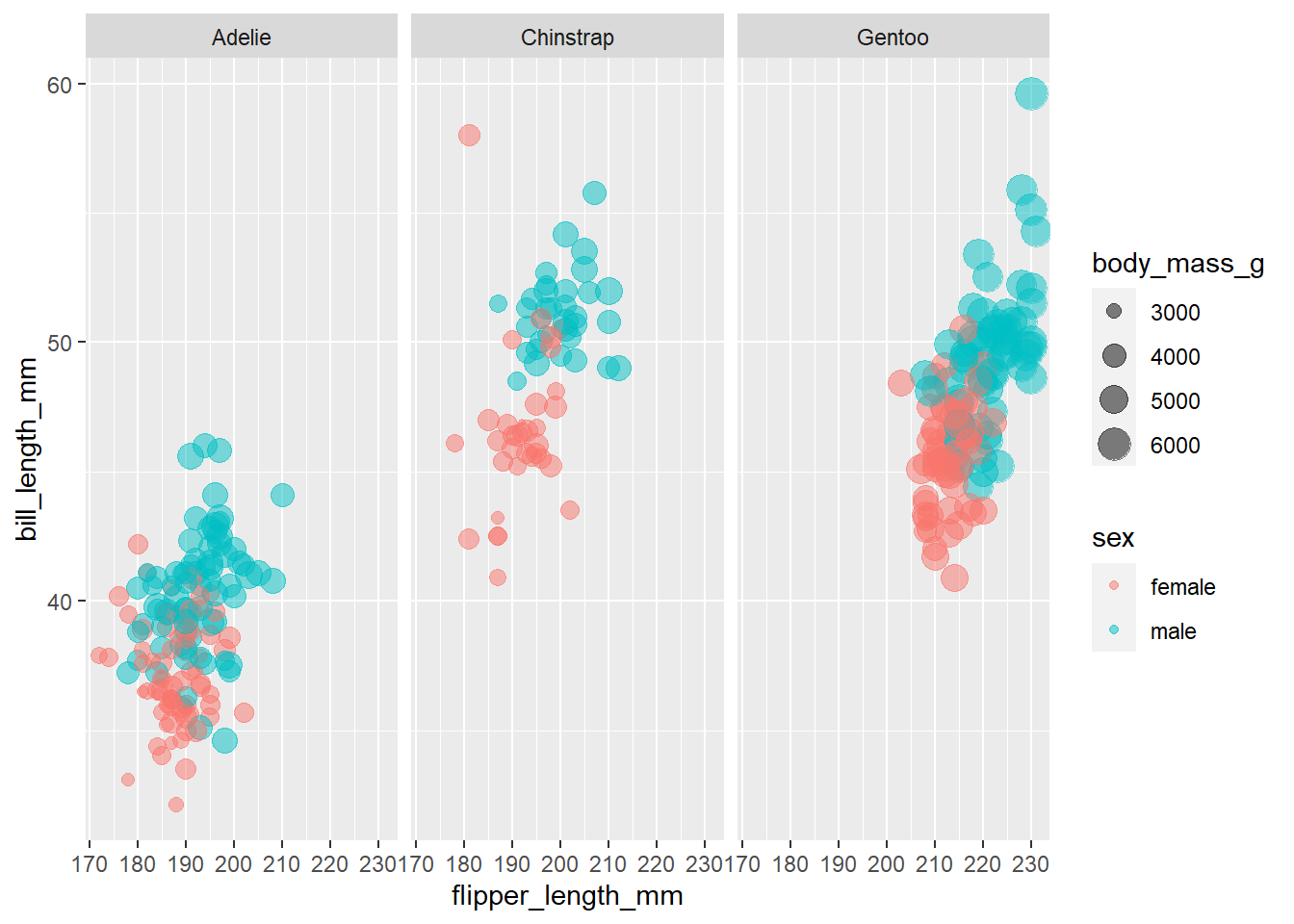
penguins_df <- penguins %>%
  filter(!is.na(sex)) %>%
  select(-year, -island)
split data 75% to traning and 25% to testing with sex as strata
set.seed(123)
penguin_split <- initial_split(penguins_df, strata = sex)
penguin_train <- training(penguin_split)
penguin_test <- testing(penguin_split)dim(penguin_train)[1] 249 6dim(penguin_test)[1] 84 6nrow(penguin_train)/nrow(penguin_test)[1] 2.964286bootstraps sample
set.seed(123)
penguin_boot <- bootstraps(penguin_train)
penguin_boot
# Bootstrap sampling
# A tibble: 25 × 2
splits id
<list> <chr>
1 <split [249/93]> Bootstrap01
2 <split [249/91]> Bootstrap02
3 <split [249/90]> Bootstrap03
4 <split [249/91]> Bootstrap04
5 <split [249/85]> Bootstrap05
6 <split [249/87]> Bootstrap06
7 <split [249/94]> Bootstrap07
8 <split [249/88]> Bootstrap08
9 <split [249/95]> Bootstrap09
10 <split [249/89]> Bootstrap10
# … with 15 more rowslogistic model
glm_spec <- logistic_reg() %>%
  set_engine("glm")

glm_spec
Logistic Regression Model Specification (classification)
Computational engine: glm randown forest model
rf_spec <- rand_forest() %>%
  set_mode("classification") %>%
  set_engine("ranger")

rf_spec
Random Forest Model Specification (classification)
Computational engine: ranger build workflow
penguin_wf <- workflow() %>%
  add_formula(sex ~ .)

penguin_wf
══ Workflow ════════════════════════════════════════════════════════════════════
Preprocessor: Formula
Model: None
── Preprocessor ────────────────────────────────────────────────────────────────
sex ~ .train logistic model
glm_rs <- penguin_wf %>%
  add_model(glm_spec) %>%
  fit_resamples(
    resamples = penguin_boot,
    control = control_resamples(save_pred = TRUE)
  )

glm_rs
# Resampling results
# Bootstrap sampling
# A tibble: 25 × 5
splits id .metrics .notes .predictions
<list> <chr> <list> <list> <list>
1 <split [249/93]> Bootstrap01 <tibble [2 × 4]> <tibble [0 × 3]> <tibble>
2 <split [249/91]> Bootstrap02 <tibble [2 × 4]> <tibble [0 × 3]> <tibble>
3 <split [249/90]> Bootstrap03 <tibble [2 × 4]> <tibble [0 × 3]> <tibble>
4 <split [249/91]> Bootstrap04 <tibble [2 × 4]> <tibble [0 × 3]> <tibble>
5 <split [249/85]> Bootstrap05 <tibble [2 × 4]> <tibble [1 × 3]> <tibble>
6 <split [249/87]> Bootstrap06 <tibble [2 × 4]> <tibble [0 × 3]> <tibble>
7 <split [249/94]> Bootstrap07 <tibble [2 × 4]> <tibble [0 × 3]> <tibble>
8 <split [249/88]> Bootstrap08 <tibble [2 × 4]> <tibble [1 × 3]> <tibble>
9 <split [249/95]> Bootstrap09 <tibble [2 × 4]> <tibble [0 × 3]> <tibble>
10 <split [249/89]> Bootstrap10 <tibble [2 × 4]> <tibble [0 × 3]> <tibble>
# … with 15 more rows
There were issues with some computations:
- Warning(s) x3: glm.fit: fitted probabilities numerically 0 or 1 occurred
Run `show_notes(.Last.tune.result)` for more information.train random forest model
rf_rs <- penguin_wf %>%
  add_model(rf_spec) %>%
  fit_resamples(
    resamples = penguin_boot,
    control = control_resamples(save_pred = TRUE)
  )

rf_rs
# Resampling results
# Bootstrap sampling
# A tibble: 25 × 5
splits id .metrics .notes .predictions
<list> <chr> <list> <list> <list>
1 <split [249/93]> Bootstrap01 <tibble [2 × 4]> <tibble [0 × 3]> <tibble>
2 <split [249/91]> Bootstrap02 <tibble [2 × 4]> <tibble [0 × 3]> <tibble>
3 <split [249/90]> Bootstrap03 <tibble [2 × 4]> <tibble [0 × 3]> <tibble>
4 <split [249/91]> Bootstrap04 <tibble [2 × 4]> <tibble [0 × 3]> <tibble>
5 <split [249/85]> Bootstrap05 <tibble [2 × 4]> <tibble [0 × 3]> <tibble>
6 <split [249/87]> Bootstrap06 <tibble [2 × 4]> <tibble [0 × 3]> <tibble>
7 <split [249/94]> Bootstrap07 <tibble [2 × 4]> <tibble [0 × 3]> <tibble>
8 <split [249/88]> Bootstrap08 <tibble [2 × 4]> <tibble [0 × 3]> <tibble>
9 <split [249/95]> Bootstrap09 <tibble [2 × 4]> <tibble [0 × 3]> <tibble>
10 <split [249/89]> Bootstrap10 <tibble [2 × 4]> <tibble [0 × 3]> <tibble>
# … with 15 more rowsrandom forest model result
collect_metrics(rf_rs)# A tibble: 2 × 6
.metric .estimator mean n std_err .config
<chr> <chr> <dbl> <int> <dbl> <chr>
1 accuracy binary 0.912 25 0.00547 Preprocessor1_Model1
2 roc_auc binary 0.977 25 0.00202 Preprocessor1_Model1rf_rs %>%
conf_mat_resampled()# A tibble: 4 × 3
Prediction Truth Freq
<fct> <fct> <dbl>
1 female female 40.5
2 female male 3
3 male female 4.96
4 male male 42.3 logistic model result
collect_metrics(glm_rs)# A tibble: 2 × 6
.metric .estimator mean n std_err .config
<chr> <chr> <dbl> <int> <dbl> <chr>
1 accuracy binary 0.918 25 0.00639 Preprocessor1_Model1
2 roc_auc binary 0.979 25 0.00254 Preprocessor1_Model1glm_rs %>%
conf_mat_resampled()# A tibble: 4 × 3
Prediction Truth Freq
<fct> <fct> <dbl>
1 female female 41.1
2 female male 3
3 male female 4.4
4 male male 42.3logistic model ROC curve
glm_rs %>%
  collect_predictions() %>%
  group_by(id) %>%
  roc_curve(sex, .pred_female) %>%
  ggplot(aes(1 - specificity, sensitivity, color = id)) +
  geom_abline(lty = 2, color = "gray80", size = 1.5) +
  geom_path(show.legend = FALSE, alpha = 0.6, size = 1.2) +
  coord_equal()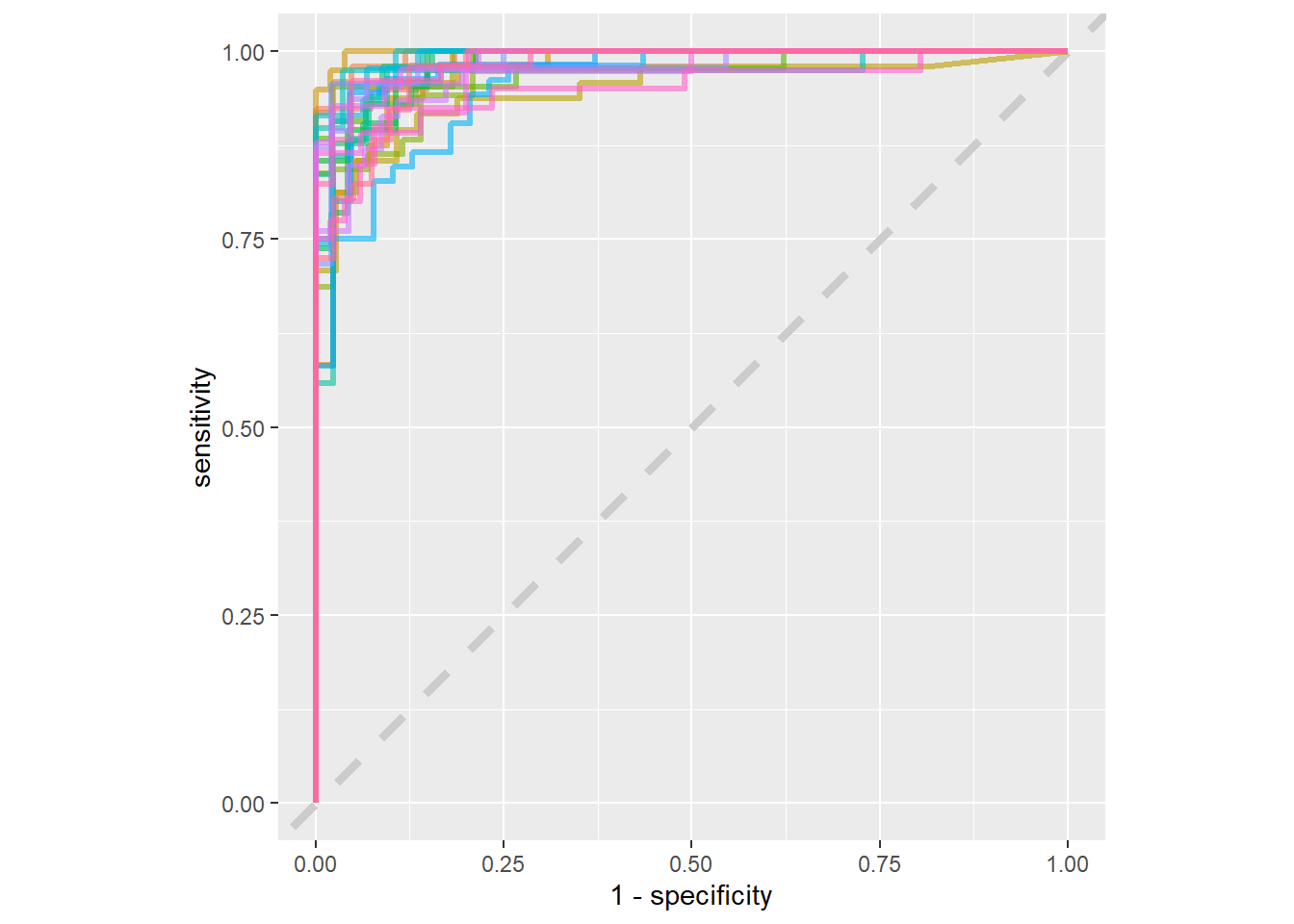
final train logistic model and fit on testing data
penguin_final <- penguin_wf %>%
  add_model(glm_spec) %>%
  last_fit(penguin_split)

penguin_final
# Resampling results
# Manual resampling
# A tibble: 1 × 6
splits id .metrics .notes .predictions .workflow
<list> <chr> <list> <list> <list> <list>
1 <split [249/84]> train/test split <tibble> <tibble> <tibble> <workflow>final fitted workflow
penguin_final$.workflow[[1]]══ Workflow [trained] ══════════════════════════════════════════════════════════
Preprocessor: Formula
Model: logistic_reg()
── Preprocessor ────────────────────────────────────────────────────────────────
sex ~ .
── Model ───────────────────────────────────────────────────────────────────────
Call: stats::glm(formula = ..y ~ ., family = stats::binomial, data = data)
Coefficients:
(Intercept) speciesChinstrap speciesGentoo bill_length_mm
-1.042e+02 -8.892e+00 -1.138e+01 6.459e-01
bill_depth_mm flipper_length_mm body_mass_g
2.124e+00 5.654e-02 8.102e-03
Degrees of Freedom: 248 Total (i.e. Null); 242 Residual
Null Deviance: 345.2
Residual Deviance: 70.02 AIC: 84.02final result:
collect_metrics(penguin_final)# A tibble: 2 × 4
.metric .estimator .estimate .config
<chr> <chr> <dbl> <chr>
1 accuracy binary 0.857 Preprocessor1_Model1
2 roc_auc binary 0.938 Preprocessor1_Model1collect_predictions(penguin_final) %>%
conf_mat(sex, .pred_class) Truth
Prediction female male
female 37 7
male 5 35final model:
penguin_final$.workflow[[1]] %>%
  tidy(exponentiate = TRUE) %>% mutate(estimate=round(estimate,4),
                                       p.value=format(p.value,scientific=F)


                                       )
# A tibble: 7 × 5
term estimate std.error statistic p.value
<chr> <dbl> <dbl> <dbl> <chr>
1 (Intercept) 0 19.6 -5.31 0.0000001100699
2 speciesChinstrap 0.0001 2.34 -3.79 0.0001482542395
3 speciesGentoo 0 3.75 -3.03 0.0024322352395
4 bill_length_mm 1.91 0.180 3.60 0.0003213825406
5 bill_depth_mm 8.36 0.478 4.45 0.0000086812196
6 flipper_length_mm 1.06 0.0611 0.926 0.3546535881832
7 body_mass_g 1.01 0.00176 4.59 0.0000044154909penguins %>%
filter(!is.na(sex)) %>%
ggplot(aes(bill_depth_mm, bill_length_mm, color = sex, size = body_mass_g)) +
geom_point(alpha = 0.5) +
facet_wrap(~species)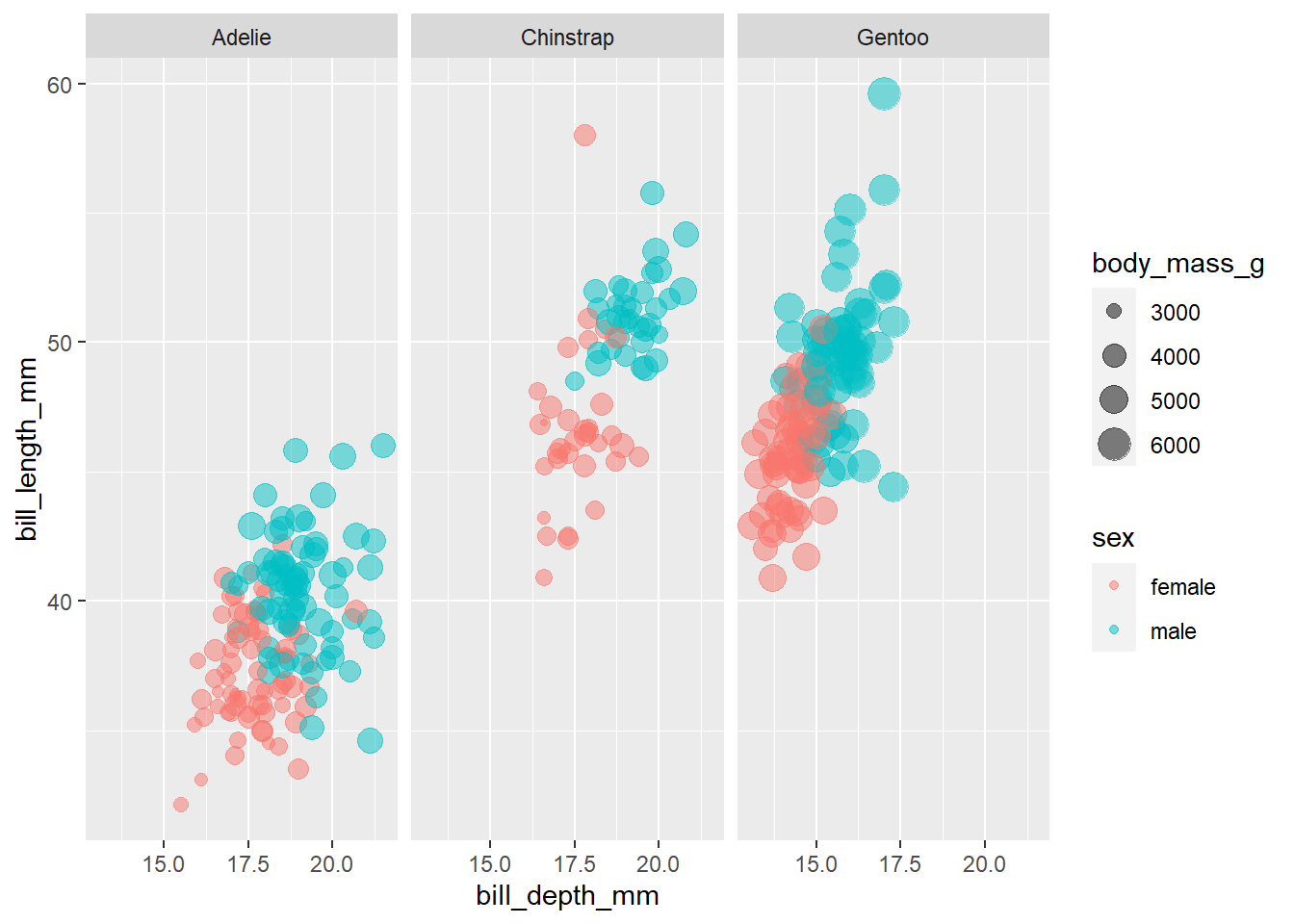
https://www.youtube.com/watch?v=z57i2GVcdww
https://juliasilge.com/blog/palmer-penguins/