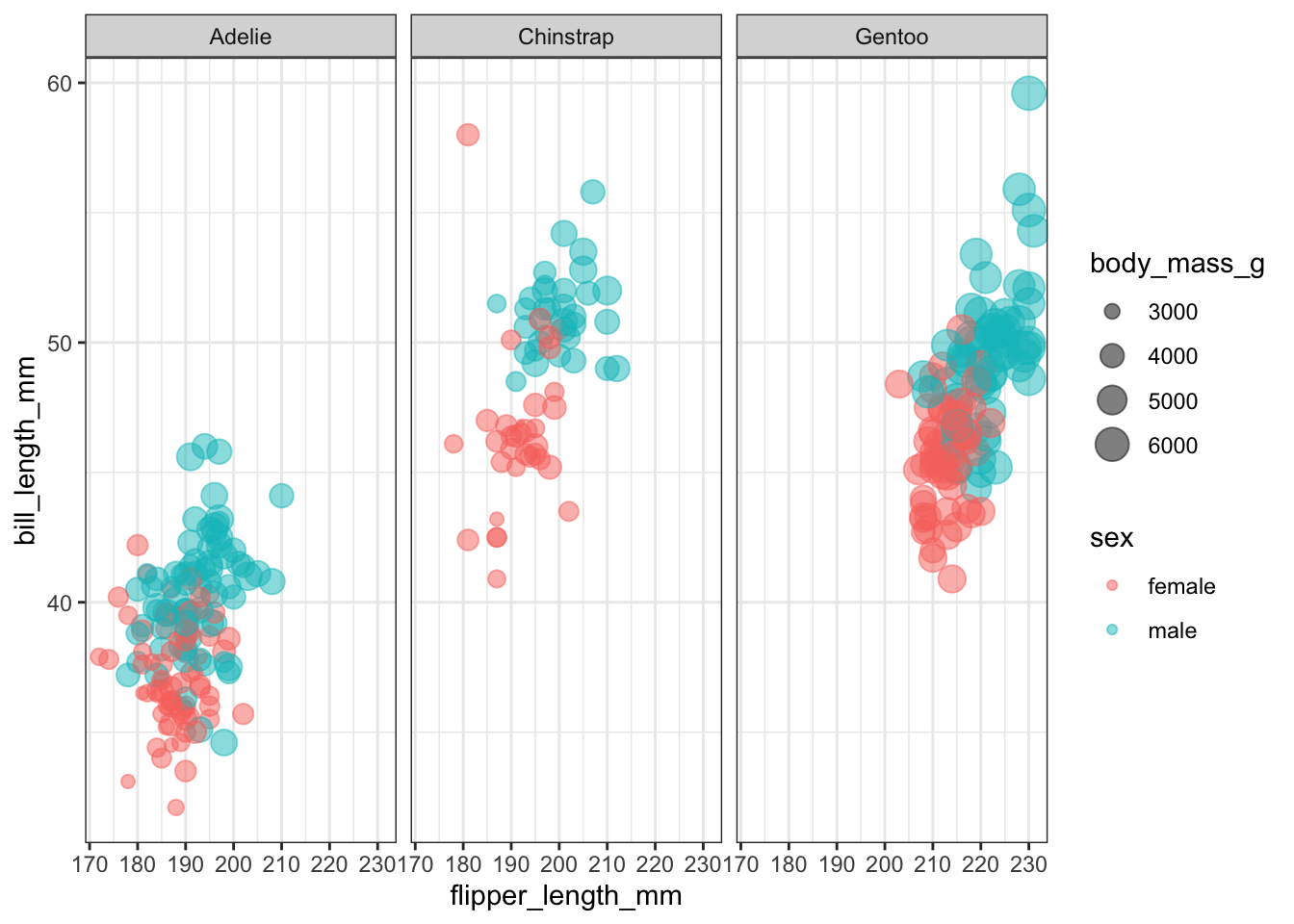
prediction for binary model

R
model
Author

Tony Duan

Published

March 9, 2024

1 load package

Load Pacakges & Set Options
library(tidyverse)      
library(tidymodels)     
library(palmerpenguins) # penguin dataset
library(gt)             # better tables
library(bonsai)         # tree-based models
library(conflicted)     # function conflicts
library(vetiver)
library(Microsoft365R)
library(pins)
tidymodels_prefer()     # handle conflicts
conflict_prefer("penguins", "palmerpenguins")
options(tidymodels.dark = TRUE) # dark mode
theme_set(theme_bw()) # set default ggplot2 theme

2 ploting

Code
penguins  %>% 
  filter(!is.na(sex)) %>% 
  ggplot(aes(x     = flipper_length_mm,
             y     = bill_length_mm,
             color = sex,
             size  = body_mass_g)) +
  geom_point(alpha = 0.5) +
  facet_wrap(~species)

3 data split

Prepare & Split Data
# remove rows with missing sex
# exclude year and island
all_penguins_df =
  penguins %>% 
  drop_na(sex) %>% 
  select(-year, -island)

# hold out 10 for final testing

hold_penguins_df=head(all_penguins_df,10)

penguins_df=tail(all_penguins_df, -10)
  
# set the seed for reproducibility
set.seed(1234)

# Split the data into train and test sets
# stratify by sex
penguin_split = initial_split(penguins_df,
                               strata = sex)
penguin_train = training(penguin_split)
penguin_test  = testing(penguin_split)

# create folds for cross validation
penguin_folds = vfold_cv(penguin_train, v = 10, strata = sex)
Code
dim(penguin_train)
[1] 242   6
Code
dim(penguin_test)
[1] 81  6

4 Create Recipe

predict sex,two category target.

Code
penguin_rec =
1  recipe(sex ~ ., data = penguin_train) %>%
2  step_YeoJohnson(all_numeric_predictors())  %>%
3  step_dummy(species) %>%
4  step_normalize(all_numeric_predictors())
1
Define the recipe on the training data with sex as the target and all other vars as predictors
2
Apply Yeo-Johnson transformation to all numeric predictors for skewness
3
Create dummy variables for nominal variable species
4
Normalize all numeric predictors

5 Specify Model

5.1 Logistic Regression

Code
glm_spec =
  logistic_reg(penalty = 1)  %>% 
  set_engine("glm")

5.2 Random Forest

Code
tree_spec =
  rand_forest(min_n = tune())  %>% 
  set_engine("ranger")  %>% 
  set_mode("classification")

5.3 Neural Network with {torch}

Code
mlp_brulee_spec =
  mlp(
    hidden_units = tune(),
    epochs       = tune(),
    penalty      = tune(),
    learn_rate   = tune()
  ) %>% 
  set_engine("brulee") %>% 
  set_mode("classification")

6 Fit Models & Tune Hyperparameters

Use Bayes optimizaiton for hyperparameter tuning

Code
bayes_control = control_bayes(no_improve = 5L,
                               time_limit = 5,# 10 mins
                               save_pred  = TRUE,
                               verbose    = TRUE)

7 Fit Models & Tune Hyperparameters

Use {workflowsets} to fit all three model types with hyperparameter optimization for random forest and neural net models.

Code
workflow_set =
  workflow_set(
    preproc = list(penguin_rec),
    models  = list(glm   = glm_spec,
                   tree  = tree_spec,
                   torch = mlp_brulee_spec)
  ) %>% 
  workflow_map("tune_bayes",
               iter      = 5L,# 5 iteration
               resamples = penguin_folds,
               control   = bayes_control
  )

8 Compare Model Results

Tabular view

Code
# create table of best models defined using roc_auc metric
rank_results(workflow_set,
             rank_metric = "roc_auc",
             select_best = TRUE) %>% 
  gt()
wflow_id .config .metric mean std_err n preprocessor model rank
recipe_torch Preprocessor1_Model2 accuracy 0.9173333 0.029470324 5 recipe mlp 1
recipe_torch Preprocessor1_Model2 roc_auc 0.9869124 0.008411554 5 recipe mlp 1
recipe_tree Iter1 accuracy 0.9046667 0.012621753 10 recipe rand_forest 2
recipe_tree Iter1 roc_auc 0.9712073 0.007699003 10 recipe rand_forest 2
recipe_glm Preprocessor1_Model1 accuracy 0.8966667 0.015513833 10 recipe logistic_reg 3
recipe_glm Preprocessor1_Model1 roc_auc 0.9634081 0.013098020 10 recipe logistic_reg 3
Code
workflow_set |> autoplot()

best model

Code
best_model_id <- "recipe_glm"

9 Finalize Fit

Code
# select best model
best_fit =
  workflow_set %>% 
  extract_workflow_set_result(best_model_id) %>% 
  select_best(metric = "accuracy")

# create workflow for best model
final_workflow =
  workflow_set %>% 
  extract_workflow(best_model_id) %>% 
  finalize_workflow(best_fit)

# fit final model with all data
final_fit =
  final_workflow %>% 
  last_fit(penguin_split)

9.1 Final Fit Metrics

Code
# show model performance
final_fit %>% 
  collect_metrics() %>% 
  gt()
.metric .estimator .estimate .config
accuracy binary 0.9012346 Preprocessor1_Model1
roc_auc binary 0.9762195 Preprocessor1_Model1

9.2 Final Fit Metrics

Code
final_fit  %>% 
  collect_predictions() %>% 
  roc_curve(sex, .pred_female) %>% 
  autoplot()

10 Create Vetiver Model & API

Create a vetiver model from final fit and upload to Microsoft one drive

Code
final_fit_to_deploy <- final_fit |> extract_workflow()

v <- vetiver_model(final_fit_to_deploy, model_name = "penguins_model",versioned = TRUE)
Code
# sign in one drive
od <- Microsoft365R::get_personal_onedrive()

# od$list_items()
board365 <- board_ms365(od, "Documents")

board365 %>% vetiver_pin_write(v)

11 download model from Microsoft one drive

Code
final_fit_to_deploy=vetiver_pin_read(board365,"penguins_model")

12 prediction

Code
glimpse(hold_penguins_df)
Rows: 10
Columns: 6
$ species           <fct> Adelie, Adelie, Adelie, Adelie, Adelie, Adelie, Adel…
$ bill_length_mm    <dbl> 39.1, 39.5, 40.3, 36.7, 39.3, 38.9, 39.2, 41.1, 38.6…
$ bill_depth_mm     <dbl> 18.7, 17.4, 18.0, 19.3, 20.6, 17.8, 19.6, 17.6, 21.2…
$ flipper_length_mm <int> 181, 186, 195, 193, 190, 181, 195, 182, 191, 198
$ body_mass_g       <int> 3750, 3800, 3250, 3450, 3650, 3625, 4675, 3200, 3800…
$ sex               <fct> male, female, female, female, male, female, male, fe…
Code
new_prediction=final_fit_to_deploy %>% predict(hold_penguins_df %>%select(-sex))
Code
glimpse(new_prediction)
Rows: 10
Columns: 1
$ .pred_class <fct> male, female, female, female, male, female, male, female, …
Code
all_penguin_test=cbind(hold_penguins_df,new_prediction)
Code
glimpse(all_penguin_test)
Rows: 10
Columns: 7
$ species           <fct> Adelie, Adelie, Adelie, Adelie, Adelie, Adelie, Adel…
$ bill_length_mm    <dbl> 39.1, 39.5, 40.3, 36.7, 39.3, 38.9, 39.2, 41.1, 38.6…
$ bill_depth_mm     <dbl> 18.7, 17.4, 18.0, 19.3, 20.6, 17.8, 19.6, 17.6, 21.2…
$ flipper_length_mm <int> 181, 186, 195, 193, 190, 181, 195, 182, 191, 198
$ body_mass_g       <int> 3750, 3800, 3250, 3450, 3650, 3625, 4675, 3200, 3800…
$ sex               <fct> male, female, female, female, male, female, male, fe…
$ .pred_class       <fct> male, female, female, female, male, female, male, fe…
Code
all_penguin_test %>% group_by(sex,".pred_class") %>% count()
# A tibble: 2 × 3
# Groups:   sex, ".pred_class" [2]
  sex    `".pred_class"`     n
  <fct>  <chr>           <int>
1 female .pred_class         5
2 male   .pred_class         5

13 reference:

https://github.com/JamesHWade/r-mlops/blob/main/the-whole-game.qmd

https://www.youtube.com/watch?v=J32pRt1nuoY